MICSA: MICs through the lens of Survival Analysis - Vivli AMR Data challenge
During the summer of 2025 I worked at Imperial College under Prof. Leonid Chindelevitch on the 2025 Vivli AMR Surveillance Data Challenge, which aims to analyze multiple large datasets of Minimum Inhibitory Contents (MICs) to extract useful learnings from the data. Bellow is the conclusions of the research in the form of a paper bellow, that can also be found on my Linkedin as a PDF.
The repository containing the work is located HERE
Authors:
- S. Nachtraba (sean.nachtrab@student.uclouvain.be)
- L. Chindelevitchb
- E. Dickensb
- W. J. Waldockc
aUniversité Catholique de Louvain, Belgium; Imperial College London, visitor bImperial College London, Department of Infectious Disease Epidemiology cImperial College London, Institute of Global Health Innovation
Made for: 2025 Vivli AMR Data Challenge
Keywords: Survival analysis, AMR, Kaplan-Meier curves, ATLAS, CABBAGE
Abstract
The collection of Minimum Inhibitory Concentrations for species-antibiotic pairs is used to track the evolution of antibiotic resistance patterns, carry out surveillance, and enable clinical decision-making by setting resistance breakpoints. Common comparison techniques for this type of data suffer from non-intuitive graphical representations and somewhat ad hoc statistical methods. In this document, we take inspiration from the field of Survival Analysis, and propose the use of its statistical methods for monitoring MIC distributions over time and space. We apply these methods to the comparison of the ATLAS dataset, provided to us in the context of the 2025 Vivli AMR challenge, with the CABBAGE dataset, collected by our group in an MRC-funded project and comprising all publicly available matching genotype and AMR phenotype data.
Objectives
Antimicrobial resistance (AMR), a pressing global issue, is monitored via the collection of minimum inhibitory concentrations (MICs) of patient samples and their comparison with clinical breakpoints established by supranational organizations (EUCAST in Europe [1], CLSI in North America [2]). The 2025 Vivli AMR data challenge aims to promote the utilization of the Vivli AMR Register, offering researchers datasets for analysis, with the goal of advancing AMR monitoring techniques.
Analytical work on large datasets is generally carried out by statisticians and computer scientists, whilst the end users of the analytical results are clinicians and public health practitioners. As a result, there may be a disconnect between the methodology used for acquiring insights from the data and the optimal framing of the knowledge for the end users.
Here we illustrate the use of Survival Analysis, an approach familiar to clinicians through its use in clinical trials [3]. For the purposes of AMR surveillance, we propose a method of MIC distribution analysis and comparison that makes use of Kaplan-Meier (KM) curves [4]. We apply them to the comparison of two datasets - the ATLAS dataset provided by Vivli and our internal CABBAGE dataset [5] - and discuss the advantages and disadvantages of this technique relative to standard approaches. Source code for our work is available in [6].
Methods
Current MIC Analysis
AMR is typically determined based on thresholds known as clinical breakpoints, which can change over time if distribution shifts are detected in the pathogen population [7]. They are set by supranational organizations (EUCAST in Europe [1], CLSI in North America [2]). When reporting AMR prevalence, the large datasets are often compressed into a single figure: the percentage of isolates classified as resistant, either by country or year, and suitable for display on timelines or maps.
Typical methods for tracking the distributional shifts of AMR suffer from a lack of interpretability and the challenges of dealing with the censorship inherent to MIC assay testing. The outputs of these methods often require knowledge outside what is usually taught in medicine, such as logistic regression modelling [8], meaning that they cannot be easily interpreted by their target users.
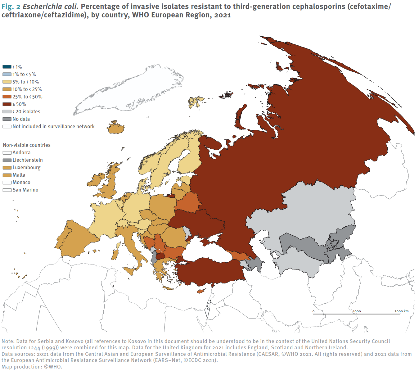
ECDC [7] Visualization methods: Left, fraction of invasive _E-Coli_ strains resistant to third generation cephalosporins in 2021, Right: Isolate quantities and percentage of resistance for Germany.
Survival analysis
Survival analysis is an area of statistics commonly used in clinical trials or other (observational or interventional) studies; its aim is to compare two or more groups on the time to an event of interest [3]. Survival analysis has the major benefit of supporting censorship (one-sided uncertainty in outcome values), which is also inherent to the process of MIC testing due to the lower limit of detection (left censoring) and upper maximum concentration (right censoring) during the serial dilution process used to measure it. Survival analysis has recognized statistical methods for estimating $p$-values (based on the null hypothesis of samples coming from the same population), and is supported by software libraries such as [9] used here, in languages such as Python [10] and R [11].
Here, we make use of survival analysis as a method for analyzing MIC values in order to obtain robust and interpretable estimations of changes, by drawing on a parallel between the time progression in classical survival analysis and the concentration increases used in MIC estimation. In both cases, the outcome of interest is the fraction of the initial population that remains alive (at a given time for the patients in a trial, or at a given concentration for the microbes in a population).
Results: Vivli AMR Challenge
To illustrate the use of Survival Analysis to compare distributions, we contrast the percentages used in the ECDC’s reports [12] in Figure 1 with a Kaplan-Meier curve comparison between years:
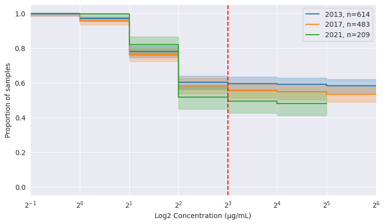
| Year | 2013 | 2017 | 2021 |
|---|---|---|---|
| n isolates | 614 | 483 | 209 |
| resistance | 60.3% | 58.2% | 51.7% |
ATLAS, number of isolates and MIC distribution for _E. coli_ tested on ampicillin in Germany. The EUCAST breakpoint at 8 µg/mL [12] is shown in red. The _x_-axis is on a log scale.
The right-hand table in Figure 2 does not make it clear whether the change in percentage is significant between years. On the other hand, the KM Curves on the left visually show a decrease in resistance. A major advantage is the toolbox of statistical tests at our disposal for deeper analysis: comparing 2017 and 2021 with 2013 using a Cox Proportional Hazards model, we get a non significant difference between 2013 and 2017, but a significant (p=0.04) difference between 2013 and 2021, allowing us to reject the null hypothesis that there is no change in hazards. The statistical toolbox at our disposal also enables a much richer analysis, which we omit here due to lack of space.
Comparison of ATLAS with external data (CABBAGE)
Survival analysis methods are also robust to distributional shifts, which we illustrate by selecting a different antibiotic, gentamicin, for the same time period (2013-2021). Figure 3 compares the ATLAS dataset to our CABBAGE dataset, currently undergoing final internal curation prior to release, which contains only isolates that have a matching genotype available [CABBAGE is yet to be published].
Figure 3 clearly shows a distributional bias in the CABBAGE dataset towards higher MIC values, confirming our suspicion that resistant isolates are somewhat more likely to get sequenced than susceptible ones. Note that this bias is less clear from the accompanying percentages (on the right).
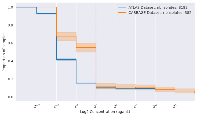
| Dataset | ATLAS | CABBAGE |
|---|---|---|
| n isolates | 8192 | 382 |
| resistance | 9.9% | 11.5% |
ATLAS and CABBAGE datasets, number of isolates and MIC distribution for _E. coli_ tested on gentamicin in the EU, 2013 to 2021. Breakpoint set at 2 µg/mL for illustration purposes.
Discussion
Making use of Survival Analysis for studying MIC distributions has a variety of advantages: a wider understanding in the scientific community, sound statistical foundations and tools available to carry out the analysis, the possibility of offering better insights into the data, and easy visualisation. However, the use of these techniques often carries some assumptions that should be kept in mind:
- In the Cox model, the assumption of proportional hazards means that a unit change in a single variable (e.g. the year or the country) always affects the risk of resistance in the same way.
- As with other areas of science, $p$-value estimation carries the potential for $p$-hacking, which can, however, be alleviated by carrying out multiple hypothesis correction (e.g. Bonferroni/FDR [14])
- The act of combining data produced with different ranges of concentrations can bias the statistical analysis. In this case, the possibility of using imputation techniques may be worth exploring.
In summary, we have shown that the use of Survival Analysis tools for MIC distributions (MICSA) is a promising approach for revealing patterns in MIC distributions across geographical and temporal shifts - showing, for instance, that a statistically significant change in E. coli’s resistance to ampicillin has happened in Germany between 2013 and 2021. MICSA can also be leveraged for comparing datasets to one another - showing that our internal CABBAGE dataset displays a significantly higher proportion of E. coli resistant to gentamicin relative to the ATLAS dataset baseline. We thus believe MICSA is a promising framework for analysing and visualising MIC distributions.
References
References
[1] “The European Committee on Antimicrobial Susceptibility Testing. Breakpoint tables for interpretation of MICs and zone diameters.” [Online]. Available: https://www.eucast.org/clinical_breakpoints
[2] “CLSI Breakpoints table, M100 ED35:2025.” [Online]. Available: https://clsi.org/shop/standards/m100/
[3] E. L. Kaplan and P. Meier, “Nonparametric Estimation from Incomplete Observations,” Journal of the American Statistical Association, vol. 53, no. 282, pp. 457–481, June 1958, doi: 10.1080/01621459.1958.10501452.
[4] S. Nachtrab, “Vivli AMR Data Challenge Survival.” [Online]. Available: https://github.com/Nachtraven/Vivli AMR Data Challenge Survival
[5] T. Cusack et al., “Impact of CLSI and EUCAST breakpoint discrepancies on reporting of antimicrobial susceptibility and AMR surveillance,” Clinical Microbiology and Infection, vol. 25, no. 7, pp. 910–911, July 2019, doi: 10.1016/j.cmi.2019.03.007.
[6] M. Aerts, K. Tzu yun Teng, S. Jaspers, and J. A. Sanchez, “A multi category logit model detecting temporal changes in antimicrobial resistance.” Accessed: Aug. 08, 2025. [Online]. Available: https://dx.plos.org/10.1371/journal.pone.0277866
[7] “Antimicrobial resistance surveillance in Europe 2023 2021 data.” [Online]. Available: https://www.ecdc.europa.eu/en/publications data/antimicrobial resistance surveillance europe 2023 2021 data 9
[8] T. G. Clark, M. J. Bradburn, S. B. Love, and D. G. Altman, “Survival Analysis Part I: Basic concepts and first analyses,” British Journal of Cancer, vol. 89, no. 2, pp. 232–238, July 2003, doi: 10.1038/sj.bjc.6601118.
[9] C. Davidson Pilon, “lifelines: survival analysis in Python,” Journal of Open Source Software, vol. 4, no. 40, p. 1317, 2019, doi: 10.21105/joss.01317.
[10] G. Van Rossum and F. L. Drake, Python 3 Reference Manual. Scotts Valley, CA: CreateSpace, 2009.
[11] R Core Team, R: A Language and Environment for Statistical Computing. Vienna, Austria, 2021. [Online]. Available: https://www.r project.org/
[12] “EUCAST Breakpoints Archive: Clinical breakpoints bacteria (v 11.0) file for screen (1 Jan 31 Dec, 2021).” [Online]. Available: https://www.eucast.org/ast_of_bacteria/previous_versions_of_documents
[13] L. Chindelevitch, “CABBAGE.” Accessed: Aug. 13, 2025. [Online]. Available: https://github.com/Leonardini/CABBAGE
[14] W. S. Noble, “How does multiple testing correction work?,” Nature Biotechnology, vol. 27, no. 12, pp. 1135–1137, Dec. 2009, doi: 10.1038/ nbt1209 1135.